 RiskAlgo
Research
One family of return distributions, three numbers — vol, skew and shape — that contains Black-Scholes and the asymmetric Laplace model as special cases. This page covers how it prices options, how its risk figures are computed, and how it is calibrated to the market.
Black-Scholes assumes the log return of a stock is normally distributed, so every strike on an expiry would have the same implied volatility. Real option markets show a smile: out-of-the-money options carry higher implied volatility than at-the-money ones, usually more so on the downside. The cause is a return distribution that is more peaked in the middle, has fatter tails, and is not symmetric.
The Q model replaces the normal distribution with the q-distribution introduced by Zhao (2024). It has exponential tails, an adjustable skew, and one extra parameter that controls how rounded the centre is. Black-Scholes, the two-parameter asymmetric Laplace model (shape 0) and everything in between live in the same three-parameter space, so one pricer, one set of risk figures and one calibration routine cover all of them.
Let \(x = \ln(S_T/F)\) up to a constant be the log return over the life of the option. Its density is
where \(s>0\) is the shape and \(\alpha,\beta>0\) are the scales of the right and left sides. Whatever the shape, the right tail decays like \(e^{-x/\alpha}\) and the left tail like \(e^{-|x|/\beta}\). Two consequences follow. All moments are finite, and the stock price has a finite expectation as long as \(\alpha<1\) (the app caps it at 0.98).
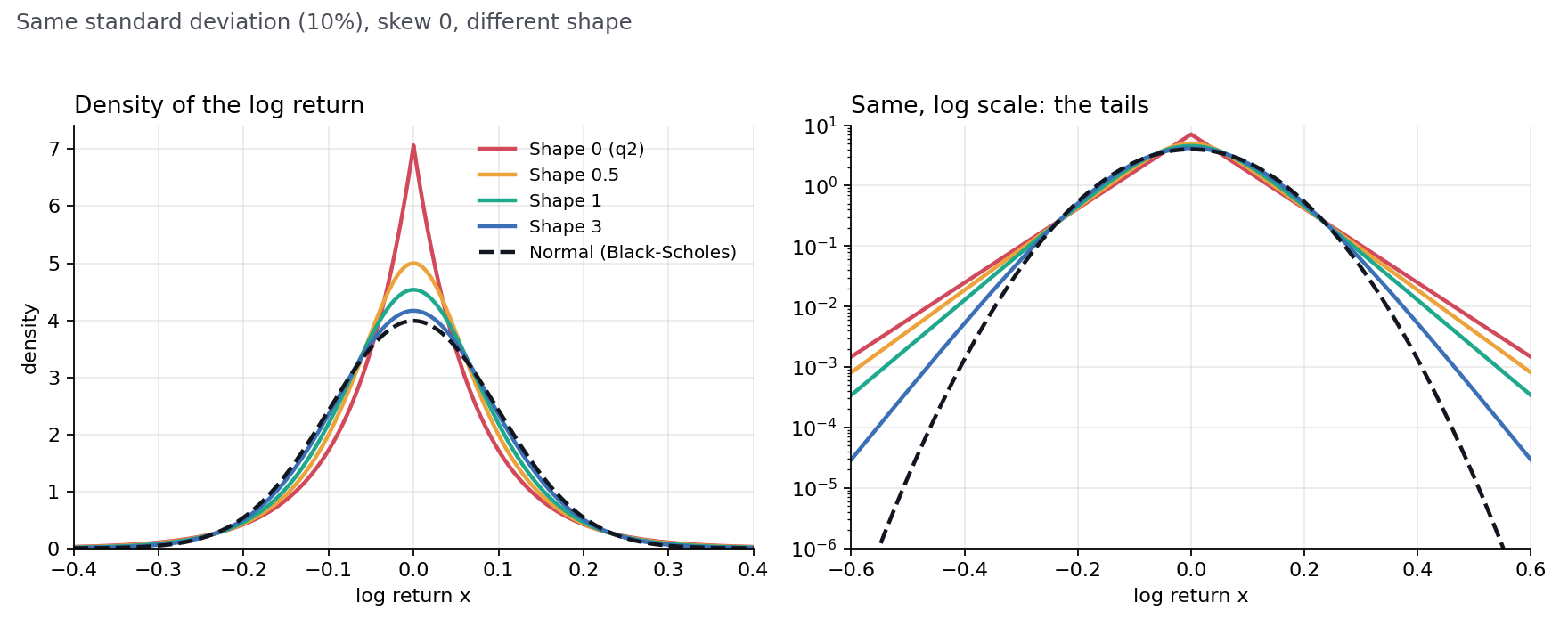
The shape \(s\) sets how the density behaves in the centre, while the tails stay exponential:
A larger shape means less excess kurtosis and a flatter smile, which is why the parameter is called shape rather than kurtosis.
The scales \(\alpha,\beta\) are not entered directly. The user-facing inputs are chosen so that vol means the same thing as in Black-Scholes:
To turn these into \(\alpha\) and \(\beta\), start from the standard law with \(\alpha_0 = \sqrt{(1+k)/2}\) and \(\beta_0 = \sqrt{(1-k)/2}\), compute its variance \(v_0\) from the three integrals \(\int x^j g\,dx\) for \(j=0,1,2\), and rescale:
For shape 0 the variance is simply \(\alpha^2 + \beta^2\), so \(c = \sigma\sqrt{T}\).
| Shape | Skew | Model | Pricing method |
|---|---|---|---|
| 0 | any | Asymmetric Laplace | Closed form |
| 0.25 to 3 | any | Q model | Gauss–Laguerre quadrature |
| 5 (Normal) | 0 (fixed) | Black-Scholes | Closed form |
Shapes below 0.25 are priced with the asymmetric Laplace closed form. In the app, selecting “5 (Normal)” fixes skew at zero and uses the Black-Scholes formula, so a price can be matched against a broker screen. A saved position therefore needs only its vol, skew and shape; no separate model name is stored.
The stock at expiry is built from the forward \(F = S_0 e^{(r-q)T}\), with \(q\) the dividend yield, and the log return \(x\):
Dividing by \(M\) makes the discounted stock a martingale, so \(E[S_T] = F\) for every skew and shape. This is the no-arbitrage condition, and it is what keeps the model consistent with put–call parity and with the market’s forward.
The stock finishes above the strike \(K\) when \(x > x^*\), where
Working through the expectation of the payoff gives, per unit of discounting,
Call, when \(x^* > 0\) (out of the money)
\[ C = e^{-rT}\,F\,\frac{e^{x^*}}{Z_1}\int_{x^*}^{\infty}\big(e^{x-x^*} - 1\big)\,g(x)\,dx \]Put, when \(x^* \le 0\) (out of the money)
\[ P = e^{-rT}\,F\,\frac{e^{x^*}}{Z_1}\int_{-\infty}^{x^*}\big(1 - e^{x-x^*}\big)\,g(x)\,dx \]The option on the other side of the forward comes from put–call parity, \(C - P = e^{-rT}(F - K)\). Always integrating the out-of-the-money side avoids subtracting two large numbers, which keeps deep out-of-the-money prices accurate.
With \(s \to 0\) the integrals are elementary. Here \(Z_0 = \alpha+\beta\), \(M = 1/\big((1-\alpha)(1+\beta)\big)\), and with \(p = \alpha/(\alpha+\beta)\) and \(\rho = K\,/\,(A F)\), where \(A = (1-\alpha)(1+\beta)\), the call value per unit of forward is
and the put follows from parity. This is the formula from Zhao (2024).
For other shapes there is no closed form, but the exponential tails make Gauss–Laguerre quadrature a natural fit:
Each integral is split into half-lines starting at 0 (for \(Z_0\), \(Z_1\) and the moments) or at \(x^*\) (for the option integral), and substituted as \(x = x_0 \pm \lambda t\). The scale \(\lambda\) is the slope of the integrand’s tail, so the remaining factor \(G(t)\) is smooth in \(t\). For the option integrals weighted by \(e^{x}\) the right-hand slope is \(\alpha/(1-\alpha)\); on the left it is \(\beta\) (with the corresponding slopes for the unweighted integrals). Exponents are combined before exponentiating, to avoid overflow in the extreme tails.
In testing, 32 nodes agree with brute-force integration to about \(2\times10^{-5}\) in price for shapes of 1 and above. The worst case, around \(10^{-3}\), is for shapes 0.25 to 0.5 with extreme vol. The strike-independent parts (the scale \(c\), \(Z_0\), \(Z_1\), \(M\)) are computed once per expiry and reused for every strike and every stock price, which makes fits and P&L scans about eight times faster.
The Q model Greeks are central finite differences on the model price:
Skew and shape are held fixed in these bumps, so the Greeks describe the model at the chosen distribution, not a smile that moves with the stock. For Black-Scholes and shape 0 the same code path is used, or the analytic formulas for Black-Scholes.
The same density that prices the options also drives the probability figures on the Pricer. The distribution of the stock price after \(T\) years is read from \(S_T = F e^{x}/M\), cut into about 800 narrow cells (equal widths in \(x\), on each side of zero). For each cell the position’s P&L is evaluated and weighted by the cell’s probability. From the resulting P&L distribution:
The tail of the stock-price distribution follows the fitted skew and shape, so a position that loses money in a large move shows a larger tail loss than under a lognormal distribution with the same vol. In Surface mode each leg takes its vol, skew, shape and implied dividend from the market surface at today’s stock price and date, and these are held fixed in the P&L analysis.
Calibration finds, for each expiry, the vol and skew (and for the ticker, a single shape) that make model prices match market quotes. The result is a surface: one \((\sigma, k)\) per expiry, a shape per ticker, interpolated linearly in time between expiries.
Before fitting, the forward for each expiry is taken from put–call parity on the quotes. For a call and a put at the same strike \(K\),
The median of these estimates over the strikes nearest the money (at least two, and only expiries of five days or more, because a small price error becomes a huge yield error over a few days) gives the forward for the expiry, and the implied dividend rate is \(q = r - \tfrac{1}{T}\ln(F/S_0)\). This captures real dividends but also borrow cost and the noise in American-style quotes, so it is a financing-adjusted forward rather than a forecast of the stock’s direction.
Only quotes that carry information about the smile are used: out-of-the-money puts below the forward and calls above it, with a two-sided market, a mid price of at least 5 cents and a bid–ask spread under 50% of the mid. Quotes more than about two standard deviations from the forward are dropped.
For one expiry the fit minimises
where \(\mathcal{V}_i\) is the Black-Scholes vega of option \(i\) and \(\sigma_0\) is a starting vol from the at-the-money option. Dividing by vega turns a price error into roughly an implied-vol error, so every quote is measured in vol points. The bell-curve factor \(n_i\) puts the most weight on strikes near the forward, which matters for the vol level: without it, noisy wing quotes pull the fitted vol above what a fit near the money would give. The minimisation is a small Nelder–Mead simplex search over \((\sigma, k)\). The reported fit error is the root-mean-square gap in vol points, normalised by \(\sum n_i^2\).
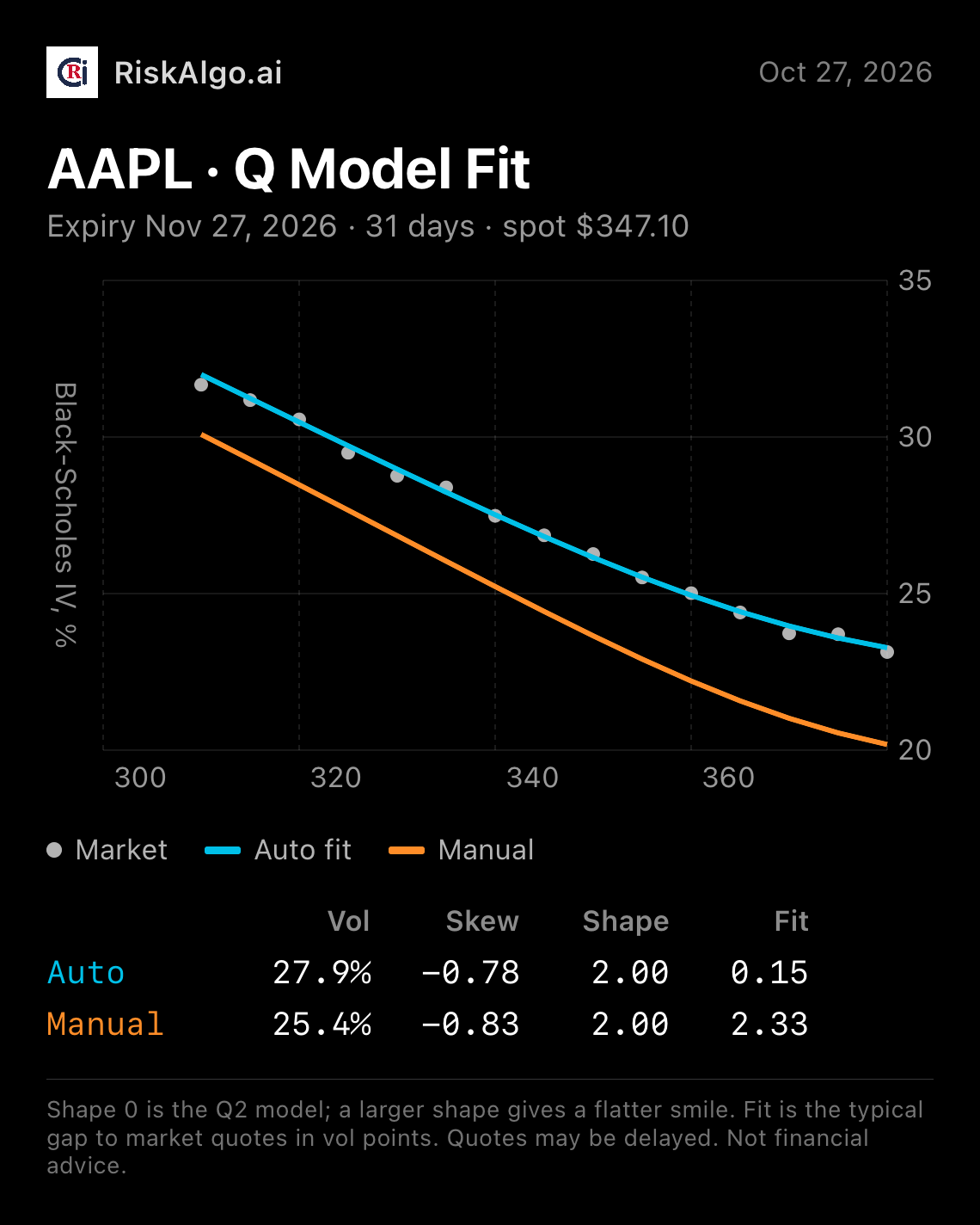
Shape is chosen once per ticker, not per expiry, from the grid \(\{0, 0.25, 0.5, 0.75, 1, 2, 3\}\):
The calibration runs in the background after quotes load; until it finishes, the app uses the shape 0 fit. The 10% hurdle prevents the extra parameter from being used to fit noise. In tests on synthetic option chains generated at shapes 0, 1 and 3, the procedure recovered the true shape each time.
Each expiry gives one fitted point, \((\sigma_j, k_j)\) at time \(T_j\). Together they form two curves over time, a vol curve \(\sigma(T)\) and a skew curve \(k(T)\). The shape \(s\) and the implied dividend are handled separately: shape is a single number for the ticker, the same at every expiry, and the dividend is a curve of its own.
Between two fitted expiries \(T_j \le T \le T_{j+1}\)
\[ \sigma(T)^2\,T = (1-\omega)\,\sigma_j^2 T_j + \omega\,\sigma_{j+1}^2 T_{j+1}, \qquad k(T) = (1-\omega)\,k_j + \omega\,k_{j+1}, \qquad \omega = \frac{T - T_j}{T_{j+1} - T_j} \]Before the first expiry and after the last, the nearest fitted value is held flat. The implied dividend is interpolated linearly in time.
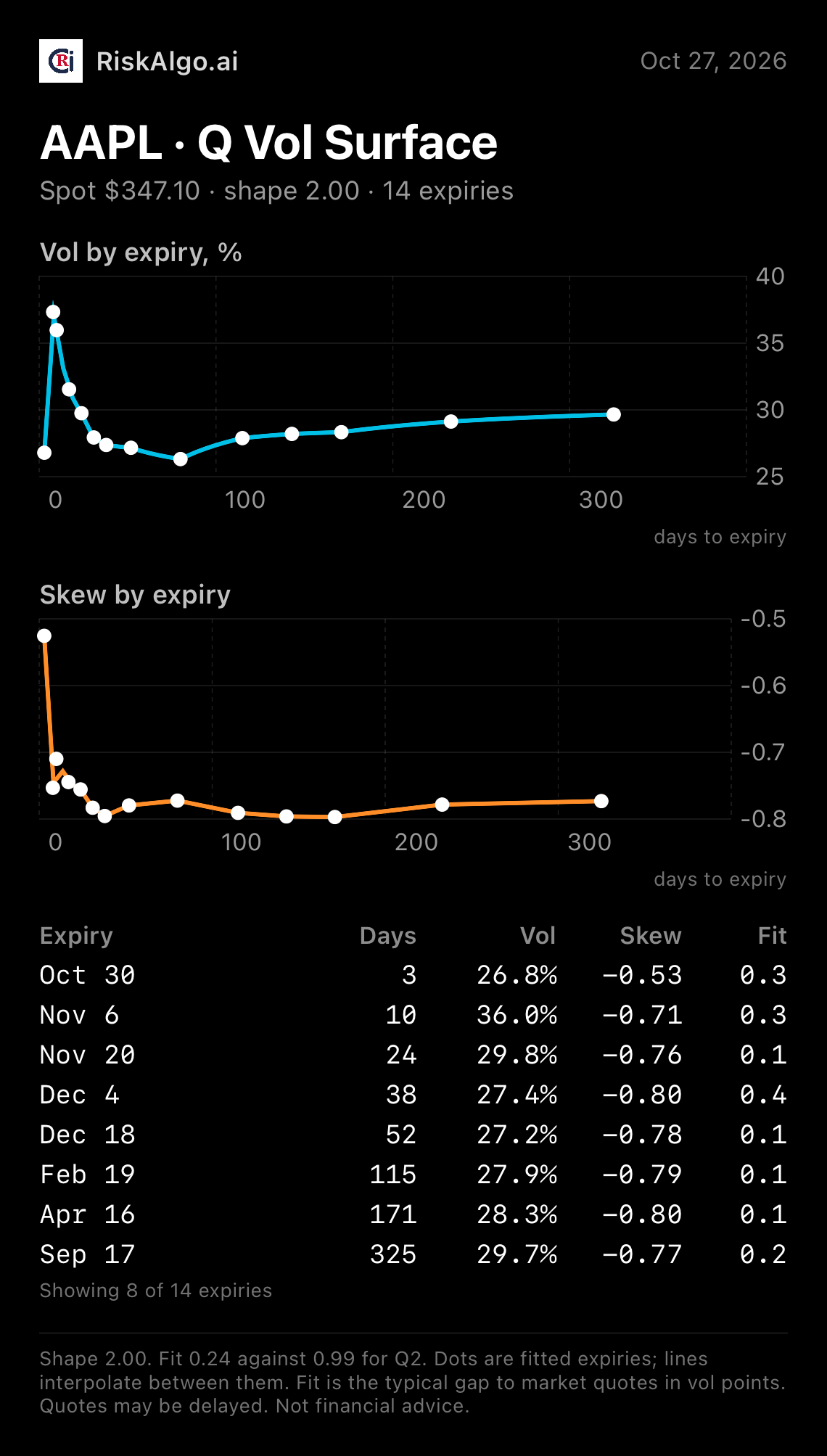
To price an option at strike \(K\) and expiry \(T\), the app reads \(\sigma(T)\) and \(k(T)\) from the curves, takes the ticker’s shape, and prices with the formulas above. The curves carry only the level and asymmetry of the distribution at that horizon. The smile across strikes at that expiry comes from the shape of the distribution itself, so no separate curve over strikes is stored.
Two points help with reading the curves. First, vol is the standard deviation of the return per \(\sqrt{T}\), so \(\sigma(T)\) is directly comparable to an at-the-money implied vol term structure. Second, skew is a property of the distribution at each horizon, and it usually moves toward zero for longer expiries, as returns summed over more days look more symmetric. The skew curve shows that, which a single skew number could not.
Vol is interpolated through total variance \(\sigma^2 T\), the standard choice, because total variance grows with time and interpolating it avoids the dips between expiries that interpolating vol directly can produce. Skew is interpolated linearly in time. The curves are therefore smooth, but they are only as good as the expiries that anchor them, so the option chain’s load-all-expiries button is useful for a well-anchored surface.
To compare model prices with the market, the Q price is converted into its equivalent Black-Scholes implied vol by solving \(P_{BS}(\sigma_{BS}) = P_Q\). The Q vol is not the same number as the Black-Scholes implied vol: it is the standard deviation of the return, while the Black-Scholes implied vol of the same option depends on strike and expiry.
This page explains the mechanics of a pricing model. It isn’t financial advice, and any model can differ from real market prices, especially around earnings or other event risk. See RiskAlgo’s Terms of Use for the full disclaimer.
Zhao’s q-distribution → the probability distribution behind the model.
Black-Scholes pricing and the Greeks → the model that sits at one corner of this space.
Risk conventions → the units and simplifying assumptions behind the Risk tab.